# 請先行安裝 Cirq: To get started we'll pip install cirq
import cirq
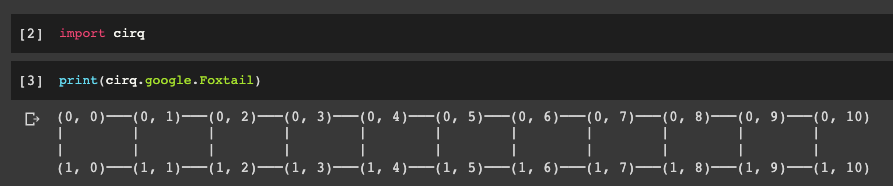
# check out a demo quantum circuit with print(cirq.google.Foxtail):
print(cirq.google.Foxtail)
2. Quantum Hello World
We're now going to define our first quantum cirquit on a quantum simulator.
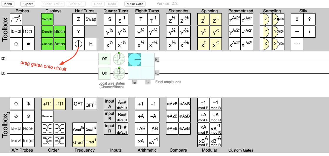
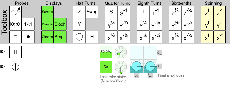
To do this we'll first visualize the circuit with Quirk, which is a quantum circuit simulator:
We can see we have two |0⟩ qubits and we can drag gates onto these circuits, which will change the output accordingly.
Jumping back to our notebook, the first step we want to do for a basic quantum circuit is define the number of qubits, logic gates, and output.
For our qubits we use the built-in GridQubit and loop through the length two times because we want to create a 3x3 row and a column matrix.
# define the length length = 3 # define the qubits qubits = [cirq.GridQubit(i, j) for i in range(length) for j in range(length)] # print the qubits print(qubits)
Now that we've created the qubits we want to add quantum logic gates to them.
Hadamard Gate
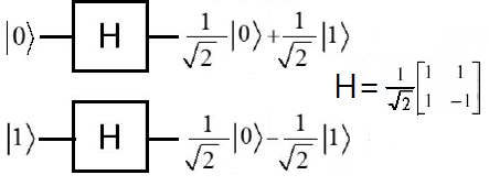
The first quantum logic gate we'll look at is the Hadamard gate, or the H-gate.
The Hadamard gate is very important because it re-distributes the probability of the all the input lines so that the output lines have an equal chance of being a 0 and 1.
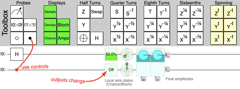
Let's go back to our simulator and drag an H-gate onto one of the |0⟩ circuits:
Now that we have the H-gate we can see the output has a 50% chance of being measured ON, or 1.
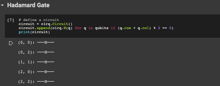
Let's now add an H-gate to all of the qubits in our circuit where the row + column index, or i + j, is even.
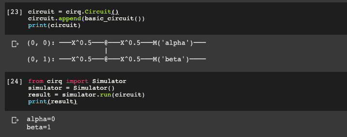
First we define a Circuit object and we are going to add to this with circuit.append.
Inside append we pass in the Hadamard gate with cirq.H(q) and loop through the qubits to check if they're even or not.
# define a circuit circuit = cirq.Circuit() circuit.append(cirq.H(q) for q in qubits if (q.row + q.col) % 2 == 0) print(circuit)
We can see we have 5 H-gates.
Pauli's X Gate
Let's now add a new gate called the Pauli X gate, which is the quantum equivalent of the NOT gate for classical computers.
A NOT gate flips the input state, so a 0 as input becomes 1 as output, and vice versa.
We can see the output of our |0⟩ circuit has is now ON, so the chance of measuring a 1 is 100%, and if we add another Pauli X gate our output becomes OFF.
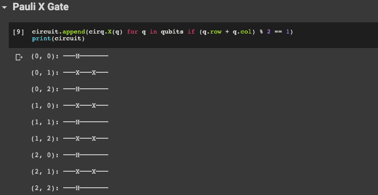
Let's noww add a Pauli X gate to our cirq circuit.
circuit.append(cirq.X(q) for q in qubits if (q.row + q.col) % 2 == 1) print(circuit)
Let's now look at how a quantum circuit is represented in Cirq.
A Cirq Circuit is made up of group of Moments, and a Moment is made up of a group of operations.
If we look at our Pauli X gate above one issue is that the H-gates and the X-gates get executed at different times.
Instead, we want both the H and X gates to be executed at the same time.
So what we're looking for is to have one Moment with both the H and X-gates.
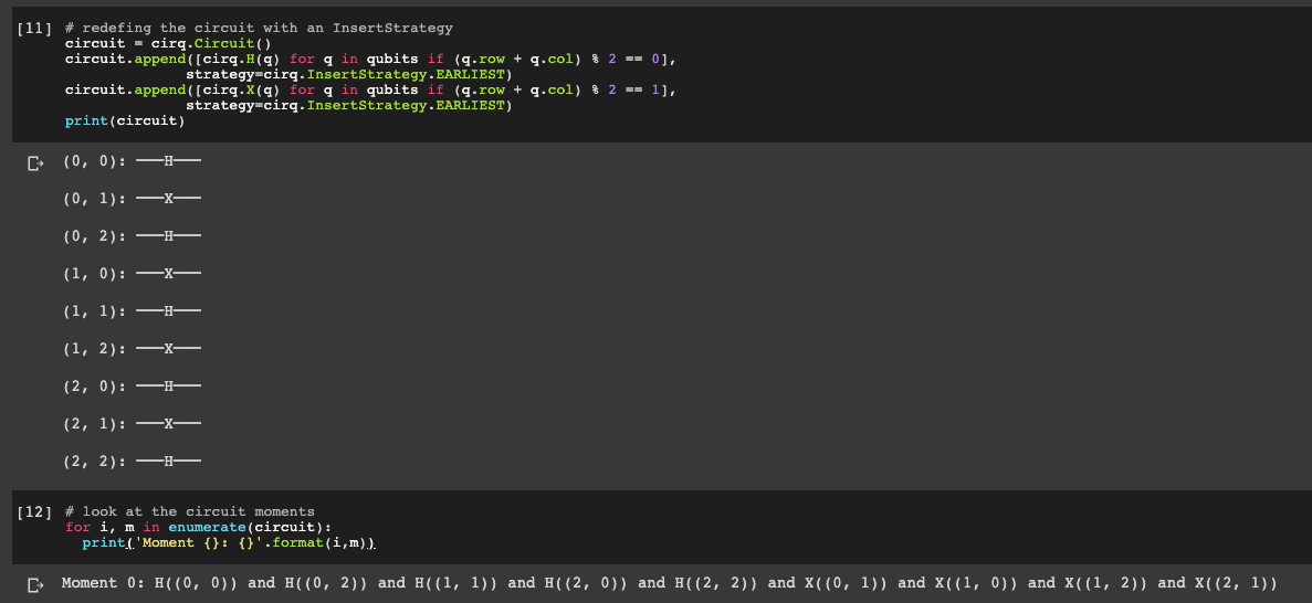
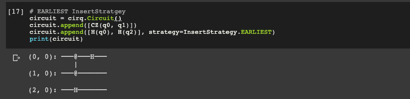
To make sure we only have one Moment we're going to set our strategy equal to cirq.InsertStrategy.EARLIEST, which governs the time of the operation execution.
# redefing the circuit with an InsertStrategy circuit = cirq.Circuit() circuit.append([cirq.H(q) for q in qubits if (q.row + q.col) % 2 == 0], strategy=cirq.InsertStrategy.EARLIEST) circuit.append([cirq.X(q) for q in qubits if (q.row + q.col) % 2 == 1], strategy=cirq.InsertStrategy.EARLIEST) print(circuit)
# look at the circuit moments for i, m in enumerate(circuit): print('Moment {}: {}'.format(i,m))
Now we can see we only have one Moment in the Circuit.
3. Creating Quantum Circuits
As mentioned, a Circuit is defined as a set of Moments.
A Moment is defined as a set of operations that can be executed on Qubits.
So to create new Circuits we need to create new Moments, which we can do with cirq.moments().
Here's what we're going to do:
We're first going to define our grid of qubits
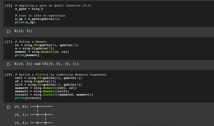
We then apply an X-gate at Qubit location (0,0)
We then turn it into an operation
We then define new Moments
We the combine Moments together to create a new circuit
# creating a grid of qubits qubits = [cirq.GridQubit(x, y) for x in range(3) for y in range(3)] print(qubits)
# applying a gate at Qubit location (0,0) x_gate = cirq.X # turn in into an operation x_op = x_gate(qubits[0]) print(x_op)
# define a Moment cz = cirq.CZ(qubits[0], qubits[1]) x = cirq.X(qubits[2]) moment = cirq.Moment([x, cz]) print(moment)
The term Fourier transform refers to both the frequency domain representation and the mathematical operation that associates the frequency domain representation to a function of time.
In simpler terms, a Fourier transform converts a single energy distribution into its constituent energy.
For example, a musical chord can be expressed in terms of the volume and frequencies of the constituent notes.
Let's now extend this concept to a quantum circuit, here's the definition of a quantum Fourier transform:
The quantum Fourier transform is the classical discrete Fourier transform applied to the vector of amplitudes of a quantum state, where we usually consider vectors of length N:=2.
This is similar to the Hadamard gate which redistributes the entire energy distribution, except the quantum Fourier transform is distributed according to the initial energy distribution.
The quantum Fourier transform can also be seen as a way to convert data, which is encoded with frequency, and convert it into a phase representation.
A phase refers to a part of the whole, so if we have a complete phase we've completed an entire cycle.
In this example we're going to use 8 qubit states, so we will encounter a phase distribution that is divided into 8 parts.
To summarize, Fourier transform is a redistribution of energy, so when you have an output you can decode the inputs from it.
Let's now implement a quantum Fourier transform circuit with Cirq.
Defining the Hadamard Gate
We're first going to define a main() method for our app
Inside the main() method we're going to create a basic circuit with 4 qubits qft_circuit
We create the 4 qubits with our generate_2x2_grid() method and then define the Circuit
Inside the Circuit we pass in the operations that will be used for to create the circuit, which are a series of Hadamard operation H(a) and then the CZ swap operations cz_swap on the qubits
We then pass in the InsertStrategy.EARLIEST as the strategy and then return the circuit
We're then going to create a simulator, pass in the qft_circuit and print the final result using numpy
import numpy as np import cirq def main(): qft_circuit = generate_2x2_grid() print("Circuit:") print(qft_circuit) # creating a simulator simulator = cirq.Simulator() # pass in the circuit and print the result result = simulator.simulate(qft_circuit) print() print("Final State:") print(np.around(result.final_state, 3)) def cz_swap(q0, q1, rot): yield cirq.CZ(q0, q1)**rot yield cirq.SWAP(q0, q1) def generate_2x2_grid(): a,b,c,d = [cirq.GridQubit(0,0), cirq.GridQubit(0,1), cirq.GridQubit(1,1), cirq.GridQubit(1,0)] circuit = cirq.Circuit.from_ops( cirq.H(a), cz_swap(a, b, 0.5), cz_swap(b, c, 0.25), cz_swap(c, d, 0.125), cirq.H(a), cz_swap(a, b, 0.5), cz_swap(b, c, 0.25), cirq.H(a), cz_swap(a, b, 0.5), cirq.H(a), strategy=cirq.InsertStrategy.EARLIEST, ) return circuit if __name__ == '__main__': main()
We've now created a quantum Fourier circuit. We can now build off this algorithm to create a quantum annealer, but we'll save that for another article.
6. Summary: Quantum Programming with Cirq
In this article we looked at how to program and simulate quantum circuits with the Google's Cirq framework, which is:
A python framework for creating, editing, and invoking Noisy Intermediate Scale Quantum (NISQ) circuits.
We started by learning how to define qubits and then add quantum operations to them. We looked at several quantum gates including the Hadamard gate and Pauli's X gate.
We then discuss how to create quantum circuits. In Cirq, a Circuit is defined as a set of Moments, and a Moment is defined as a set of operations that can be executed on qubits.
We then looked at how to create a quantum simulator with Cirq.
Finally we tied all of this together by creating a quantum Fourier transform circuit and simulating in with Cirq.
In the next article we'll build on these concepts and look at programming a quantum annealer with D-Wave.